

Data analysis fifth step: data processing
The road so far
So, you started with a goal, you found some related datasets and pre-processed them; NOW! Here is where the going gets rough (so if you do not feel tough enough, please come back later ?, we won’t judge you)!
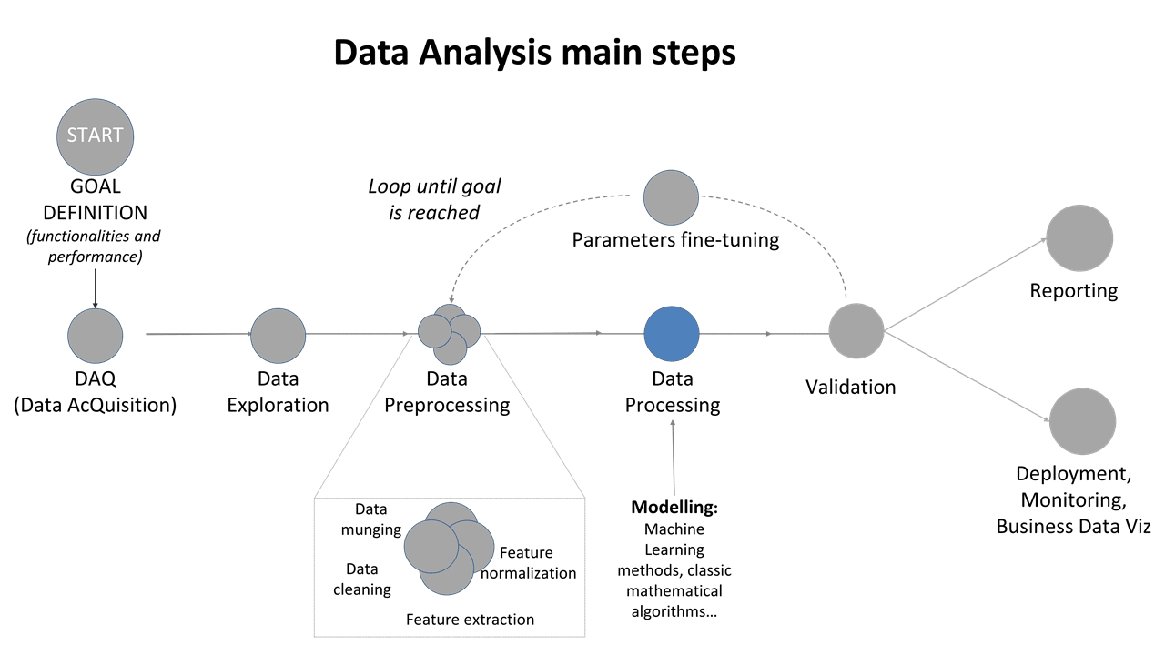
Figure 1: Data Analysis main steps: focus on data processing
The road ahead
Let’s assume that you, interested reader, already know that the model is not the reality, but only an approximation of it. Like a map of a mountain is not the physical mountain, but a representation of it. As for the map, we need to decide the accuracy and the information we are interested on.
For the map, we could need the info of the city street by street or, maybe, we just need all the historical monuments location like in a touristic map. For a model, we want to know if our model can extract the info we need (for example, the power production of a power plant given irradiance and temperature), but also with what level of accuracy.
Thus, there are several questions to keep in mind: which are the models that can be applied successfully in this situation? Is an Artificial Intelligence approach feasible? Is a simpler mathematical method better suited?

Do not forget, at this point you need to think about how to validate your results (wait for my next post for details), otherwise you could choose a model you are not really able to interpret. That is: if you want an address information in New Delhi, you will not choose a historical map of Asia…
Finally, when choosing the model, we must also take into account our expertise in the results interpretation: if your model calculates only the MAPE and you do not know what it is, maybe you should do something about it: change method, or study more (and that depends on you, dear reader ?, not on the cheap or very expensive tool you are using!).
Thus, the key words here are “quantitative” and “interpretability”.
Nowadays, we can group two kinds of approaches of models, one that we’ll call as domain-driven (mathematical-physical models) and data-driven approach (standard statistical or artificial intelligence models).
The first kind of model, domain-driven, is related to the ability and expertise of the model-creator to mathematically describe the physical components of the phenomenon. For example, taking a photovoltaic plant, you should be able to describe what happens from the cell to the inverter, typically using manufacturer information to characterize the model parameters; the deeper the domain knowledge, the more the plant model will be effective. The PROs of this domain-driven approach are the human-interpretability of the results, the capability of improve the models when the expertise increases, and the possibility to create a model without archive data from the plant (for example, if the plant is not yet built, or it is at young stage of its operative life). The CONs are that, especially for large PV plants, it is not always possible to accurately describe all components, leading often to the necessity of post-processing model raw outputs to fine-tune the results. Example of this kind of approaches, schematically, are “SAM“, “PVsyst“, “PVLib“.
Data-driven approaches are typically based on standard statistical procedures such as polynomial regression, best fitting approaches, MonteCarlo simulation or Artificial Intelligence algorithms such as neural networks or decision trees.
These models simulate the behavior of the plant based on an archive of data used to assess the model parameters (in the context of machine learning, this step is called training of the model using the training dataset). The CONs are that in order to obtain reliable outputs, a suitable data archive is required in order to correctly compute the models’ parameters: the data archive must be large enough to be representative of all the working conditions (e.g. in the solar area, one year of data is the minimum needed to be able to follow the sun conditions), and must not contain anomalous data (for example, if periods of plant malfunctioning are in the training dataset of a machine learning algorithm, the system will “learn” these conditions as nominal, and the outputs will not be reliable).
Real-world example
As a real-world example, we will show how to use a dataset of irradiance and power data of a given photovoltaic power plant to calculate the power production. We will do it via different approaches: using a simple linear approximation, using a more sophisticated opto-electronic model and using a regression by a neural network. At the end, we will see that they are not so different in the results, and even in the interpretation (if you are curious and want to go the extra-mile, we will also open up the machine learning black box!).
So, let’s start. The dataset is composed by irradiance and power data for a power plant in Sicily for the 2019 year [1]. We also know the basic as built of the plant, that is how and what kind of inverters and panels are installed, and tilt and azimuth information. First of all, we decide the goal: since we do not need extreme accuracy, we decide to create a very preliminary model using only a simple “y = a*x + constant” regression, where “x” is the irradiance and “y” is the power. Given the dataset extension, we divide it in two subsamples, one for “training” (January -> October) and one for “testing” (November -> December). These terms are borrowed from the machine learning world, and depending on the working area habits they may change. To be as general as possible, let’s say the training dataset is where you do experiments and build the model, while the test dataset where you look at results.
For the regression, we will use the python “statsmodels” package, being user-friendly and with a lot of statistical information useful for the interpretation. As a pre-processing, we just removed very low irradiance data < 100 W/m^2 and power data lower than 20 W.
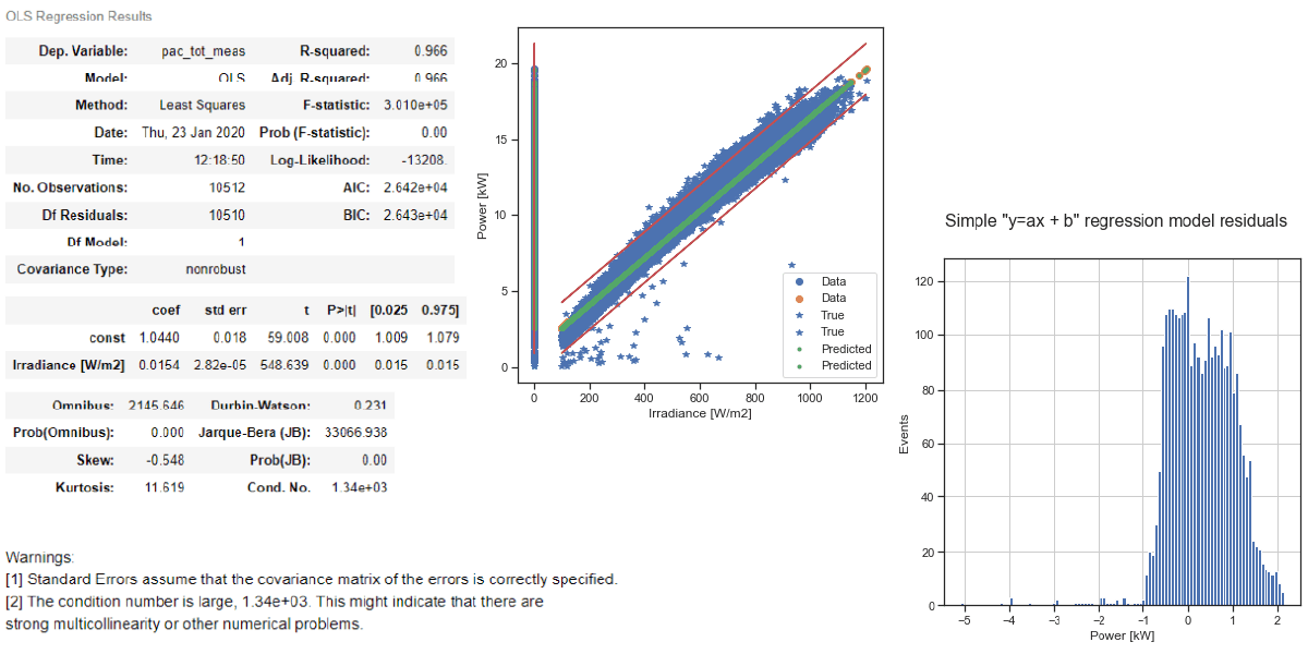
Figure 2: simple regression “y= ax + constant” using the python statsmodels package
We calculate the mean absolute error (MAE) and we got 0.6. Without going into details, we can see from the tables and the plots that the approximation is very simple, and does not take into account the shape of the irradiance-power curve, especially the non-linear parts for low irradiance and high irradiance. Still, it can be useful as an initial starting point.
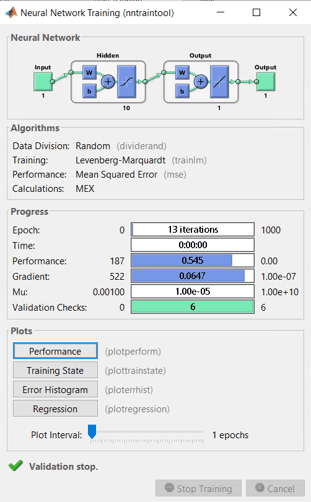
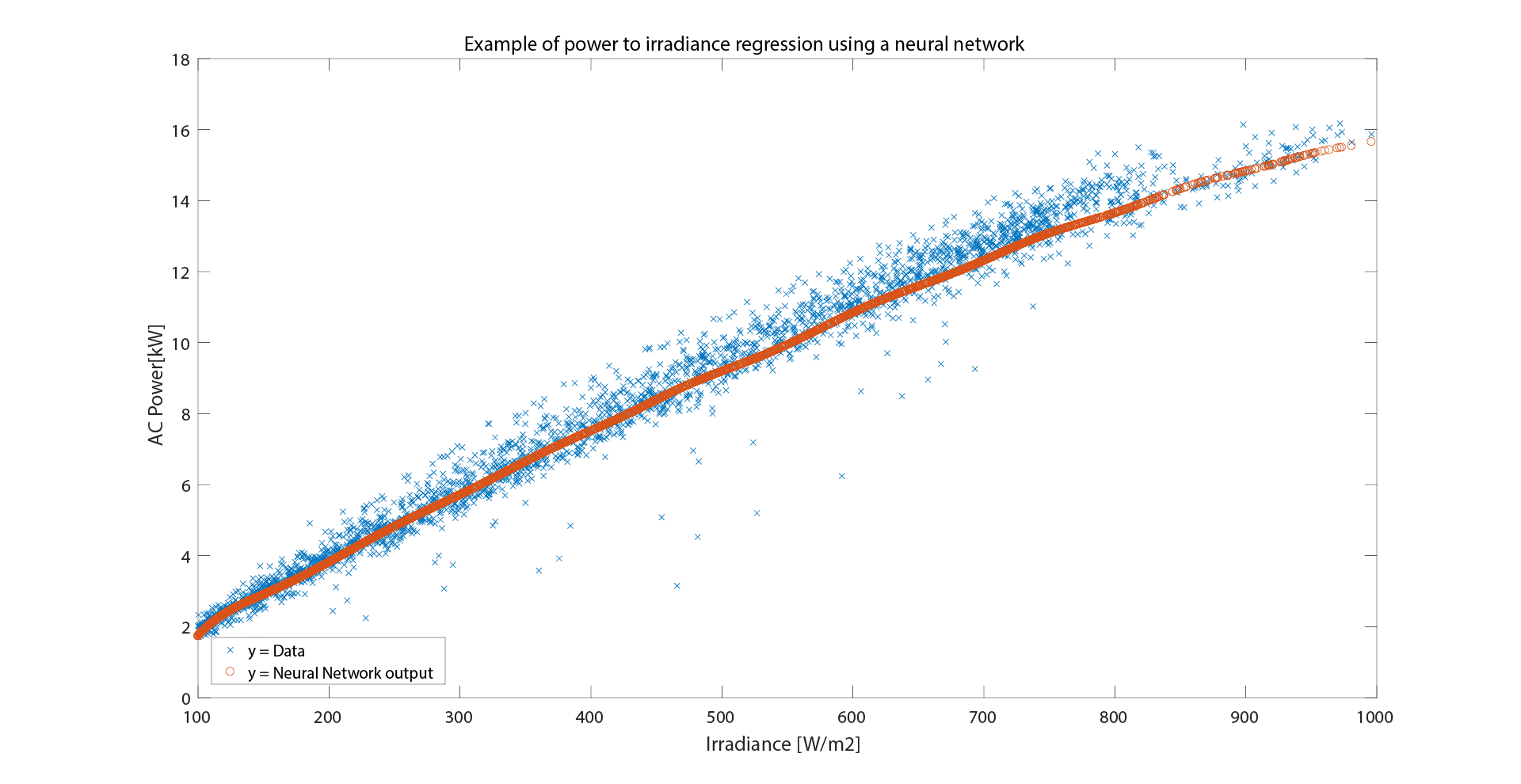
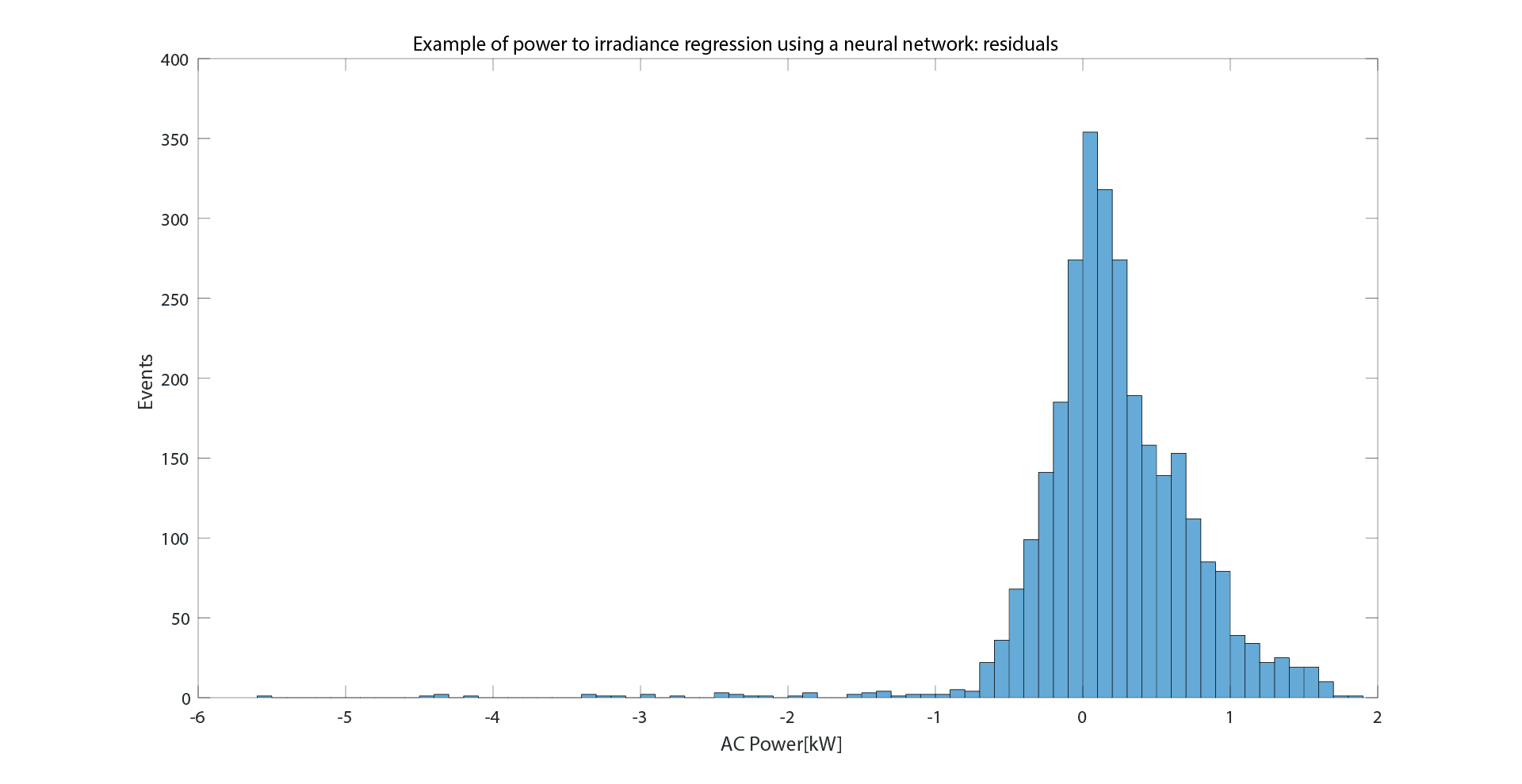
Then, we decide to be more accurate and we use a neural network approach. To be able to do a fair comparison, we will use the same data and same training-test division. We used of the most basic architecture and tool available in MatLab, that is the “feedforwardnet” with all parameters left to default. After the training, in the test dataset we obtained a MAE = 0.4, and from the plots you can see how the function is more accurate in reproducing the shape of data, and also the residual distribution has a better bell-like shape, as you would basically expect a-priori.
Then, we can do a final example (well, there is no two without three…) using physical model reproducing the plant behaviour, starting from an inverter model up to an opto-electronic model reproducing the behaviour of the solar cell. This would be particularly useful, as described, when you DO have knowledge of the power plant, but you DO NOT have historical dataset where to train a machine learning or a regression algorithm. In this case, the results are worse than the previous approaches, with a MAE of about 1.0 and very large residual distribution.
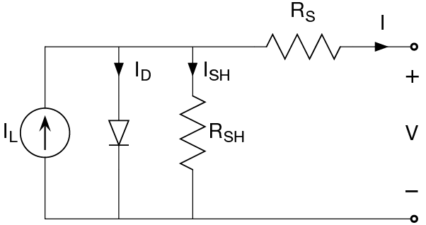
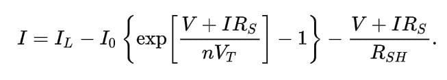
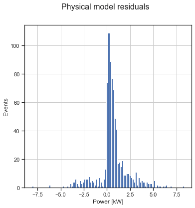
Figure 3: The equivalent circuit of a solar cell and the main formula relating solar cell parameters to the output current and voltage, from https://en.wikipedia.org/wiki/Theory_of_solar_cells
Putting all together:
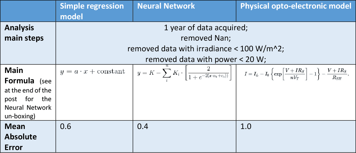
Table 1: resume of the different approaches’ characteristics
Lesson Learned becomes tip and tricks!
- Skimming dataset and testing progressively to have a preliminary idea of how many seconds -> hours the full code will need to run;
- When the modelling is difficult, make a toy-model (a simplified model to see if assumptions turns out fine), then, once the activity is clearer, make a real model;
- Modelling timings;
- Kind of personal computer where to run code (CPU, RAM);
- Parallelizing tip and tricks;
- After having choose the model, you could need to go back and do some preprocessing again (for example, some neural network appreciates normalized inputs).
When everything else fails
Use a Gaussian: using gaussian-based model can be the last option, when you have no idea what kind of distribution you would expect, or when other approach seems not working. When everything else fails, it is a rough but reasonable approximation of almost every natural, artificial or human phenomenon.
BONUS: If one Gaussian fails, use more Gaussians!

Useful and most used tools
R, SAS, SPSS, python, Julia, Rapidminer, MatLab, Weka, Scala, ROOT (Cern), C, C++, Knime and all the related application such as Tensorflow, Keras…
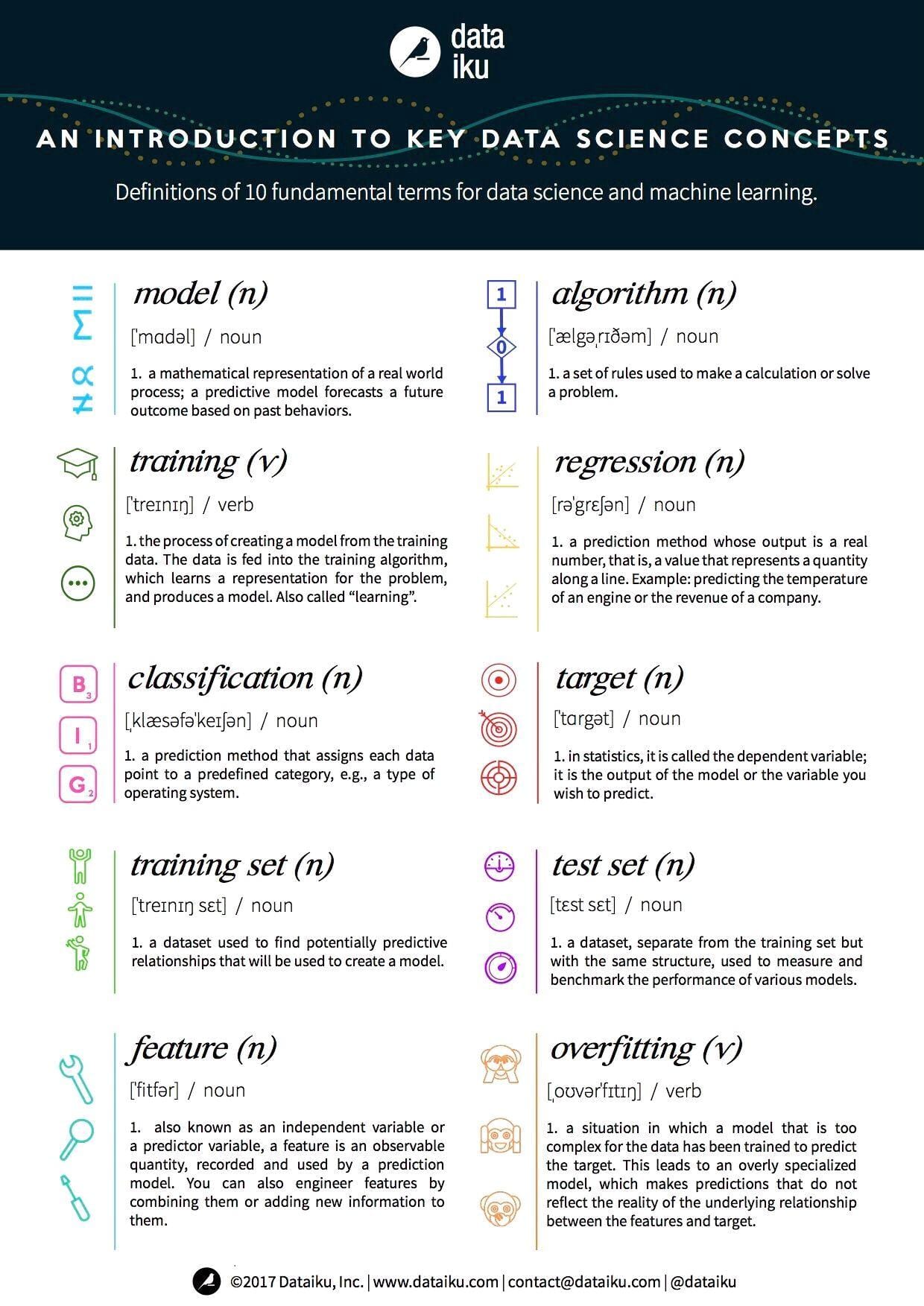
Just to make a brief introduction, some very preliminary definition I found usefully are collected by dataiku in the figure.


Bonus: opening the black box
Schematically, Machine Learning approaches are used the best when we do not have a deep knowledge of a problem that is highly non-linear. Thus, we task the “learning” step to modify the initial architecture and features of the approach (for example, the neural network number of neurons, layers and weights) to best fit the training dataset. Sometimes we just forgot that, in the end, a computer is just a very efficient calculator, and it is just dealing with more or less complex mathematical functions. In the above example, the Neural Network explicit formula is just:
(((2/(1+exp(-2*(x1*-1.346617e+01 + 1.444347e+01)))-1)*-2.109103e-01 +
(2/(1+exp(-2*(x1*1.454931e+01 + -1.043638e+01)))-1)*1.145440e-01 +
(2/(1+exp(-2*(x1*1.305265e+01 + -6.722161e+00)))-1)*3.747793e-02 +
(2/(1+exp(-2*(x1*-8.381731e+00 + 2.601264e+00)))-1)*-8.969784e-02 +
(2/(1+exp(-2*(x1*7.909794e+00 + -3.337153e-01)))-1)*1.264497e-01 +
(2/(1+exp(-2*(x1*9.855086e+00 + 1.989964e+00)))-1)*9.270696e-02 +
(2/(1+exp(-2*(x1*8.223900e+00 + 3.416464e+00)))-1)*1.036186e-01 +
(2/(1+exp(-2*(x1*6.953288e+00 + 4.468370e+00)))-1)*1.424730e-01 +
(2/(1+exp(-2*(x1*8.047376e+00 + 7.021552e+00)))-1)*1.157003e-01 +
(2/(1+exp(-2*(x1*-1.298737e+01 + -1.449689e+01)))-1)*-6.501161e-01 + -3.973539e-01))
That is, very long and with a lot of numbers, but we have seen worse…?!!!
Notes
[1] We would like additional data, given that the sun typical time-interval is one year, so we prefer having 5 or 10 years. Unfortunately, sometimes you need to work with what you got… (See reference)For the curious costumer
At i-EM S.r.l., we think that a long journey starts from a single and smart step; also, we know that the devil is in the details, and a good procedure can help to take them into account.
For the keen reader
Some further readings I found interesting (not so much as my post, sorry for you…)
- Machine Learning Explained: Algorithms Are Your Friend: https://blog.dataiku.com/machine-learning-explained-algorithms-are-your-friend
- Commonly used Machine Learning Algorithms (with Python and R Codes) https://www.analyticsvidhya.com/blog/2017/09/common-machine-learning-algorithms/
- Which machine learning algorithm should I use? https://www.datasciencecentral.com/profiles/blogs/which-machine-learning-algorithm-should-i-use
- What is the Difference Between a Parameter and a Hyperparameter? https://machinelearningmastery.com/difference-between-a-parameter-and-a-hyperparameter/
Author

Fabrizio Ruffini, PhD
Senior Data Scientist at i-EM